Processes

Inference

During the inference process, machine learning models create a heatmap of the input images.

Before the image is processed, a benchmark is run on the GPU to determine the largest tile that can fit into memory. Then, the image is divided into tiles of the determined size (including a small portion of context). Next, the inference process is run, and the results are saved on the disk. When all tiles are finished, they are merged into the final resulting mask. The tiles are then deleted.

Input RequirementsExpected Output

• The only supported image formats are Geotiff files (.tif / .tiff)
• The image needs to have at least three channels (RGB - red, green, blue).
• It is strongly recommended that the image size is less than 25GB.
• The image must be georeferenced. This includes among other things: coordinates for top left corner; number of pixels for width and height; and resolution.
• It is recommended to use cloud optimized geotiff (COG) files. Although inference will work with standard Geotiff files with the above specifications, performance may suffer significantly if the image is not tiled.
• The filename should not be longer than 120 characters or include any special characters.

• Geotiff file (.tif / .tiff)
• Single-channel mask with positive values representing target detection class features
• Heatmap of the given detection class depicted in 8-bit grayscale
• Heatmap pixel values from 0-255
• Output can be used as input in vectorization or other Orca processes
• Raster data

Vectorization

Vectorization reads the grayscale raster data produced by the inference process and produces output in the form of polygons. The output vector data will be in the same coordinate system as the input. The resulting polygons and coordinate system information are saved in the geopackage file. To provide building footprints only model BSHRK-W-BFD-11 currently utilizes vectorization. This process may not be useful for or supported by other detection classes.

Input RequirementsExpected Output

• Geotiff file (.tif / .tiff)
• Results from inference process
• Raster data

• GeoPackage file (.gpkg)
• Regularized polygons representing outlined detected feature
• Vector data

For more information on vectorization see Orca Configuration in the usage guide.

Orca Usage.

Polygon Creation and Simplification

For each connected region of high-confidence pixels, a polygon is created. The polygons are oriented counter-clockwise (points of the outer ring are counter-clockwise and points of holes are oriented clockwise). This ensures that the signed area of the polygon is positive.

The polygons are then processed using the Douglas-Peucker simplification algorithm. Polygons that have an area below 10m² are discarded. The polygons are then regularized producing more standard architectural shapes. If, due to feature complexity, the regularization process results in a polygon that is too different from the results prior to regularization, the vectorization process will revert back to the results created by the Douglas-Peucker algorithm (see fig. 1). In most cases the results after regularization are more accurate, however it is possible that smaller features with curved edges will be rendered as rectangular (see fig. 2).

Although an attempt is made to ensure valid polygon geometry, in some rare cases an invalid polygon cannot be repaired by the algorithm. Therefore, if guaranteed valid geometry is required, checking the validity of resulting polygons using standard GIS software such as OGR is recommended.

fig. 1 - footprint is more accurate prior to regularization.

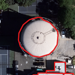
^{_{(Input imagery by Vexcel Imaging GmbH)}}

 

 

fig. 2 - small round object is shown with four right angles.

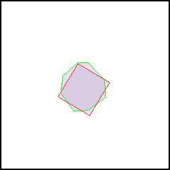
Image Tiling

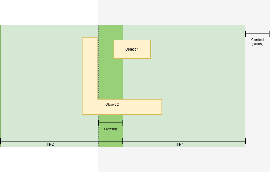
To produce a faithful vectorized image, the image is divided into tiles. Regardless of tile size, 300m of context is added to each side of a tile. This means that any given tile will overlap with neighboring tiles by 300m in all four directions.

To avoid overlapping polygons, in the majority of cases a polygon will be discarded if the central point (centroid) of the polygon lies within the tile and not within the context area.

Due to this process two known issues arise:

1. Maximum feature size is limited to 600m for any one possible dimension (length, width, diagonal).
2. Irregularly shaped features near to context areas limits may be divided and output as overlapping objects due to insufficient context. (see fig.3)

fig. 3 - Object 1 will be included in tile 1. Object 2 will erroneously be included in tile 1 and the adjacent tile 2 to the left as two distinct, but overlapping, objects.

Segmentation

For some detection classes (roads, clouds, etc.), it is desirable to produce binary outputs. During the segmentation process the 256 possible values of the 8 bit grayscale heatmap produced by the inference process are simplified to two values.

To achieve this, the segmentation process evaluates the heatmap against a set threshold value. Any pixel with a value higher than the threshold value is assigned a value of 1 (detected object); any pixel below the threshold value is assigned a value of 0 (no object detection).